转载来源:http://blog.csdn.net/bamboolsu/article/details/49313379
Webrtc 中的带宽自适应算法分为两种:
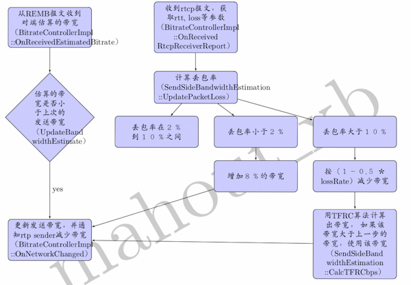
1. 发端带宽控制, 原理是由 RTCP 中的丢包统计来动态的增加或减少带宽,在减少带宽时使用TFRC 算法来增加平滑度。
2. 收端带宽估算, 原理是并由收到 RTP 数据,估出带宽; 用卡尔曼滤波,对每一帧的发送时间和接收时间进行分析, 从而得出网络带宽利用情况,修正估出的带宽。
两种算法相辅相成, 收端将估算的带宽发送给发端, 发端结合收到的带宽以及丢包率,调整发送的带宽。
下面具体分析两种算法:
1. 发送端带宽控制
2. 接收端带宽估算算法分析
结合文档http://tools.ietf.org/html/draft-alvestrand-rtcweb-congestion-02以及源码webrtc/modules/remote_bitrate_estimator/overuse_detector.cc进行分析。
带宽估算模型: d(i) = dL(i) / c + w(i) d(i)两帧数据的网络传输时间差,dL(i)两帧数据的大小差, c为网络传输能力, w(i)是我们关注的重点, 它主要由三个因素决定:发送速率, 网络路由能力, 以及网络传输能力。w(i)符合高斯分布, 有如下结论:当w(i)增加是,占用过多带宽(over-using);当w(i)减少时,占用较少带宽(under-using);为0时,用到恰好的带宽。所以,只要我们能计算出w(i),即能判断目前的网络使用情况,从而增加或减少发送的速率。
算法原理:即应用kalman-filters(卡尔曼滤波)
theta_hat(i) = [1/C_hat(i) m_hat(i)]^T // i时间点的状态由C, m共同表示,theta_hat(i)即此时的估算值
z(i) = d(i) – h_bar(i)^T * theta_hat(i-1) //d(i)为测试值,可以很容易计算出, 后面的可以认为是d(i-1)的估算值, 因此z(i)就是d(i)的偏差,即residual
theta_hat(i) = theta_hat(i-1) + z(i) * k_bar(i) //好了,这个就是我们要的结果,关键是k值的选取,下面两个公式即是取k值的,具体推导见后继博文
E(i-1) * h_bar(i)
k_bar(i) = ——————————————–
var_v_hat + h_bar(i)^T * E(i-1) * h_bar(i)
E(i) = (I – K_bar(i) * h_bar(i)^T) * E(i-1) + Q(i) // h_bar(i)由帧的数据包大小算出
由此可见,我们只需要知道当前帧的长度,发送时间,接收时间以及前一帧的状态,就可以计算出网络使用情况。
接下来具体看一下代码:
 1void OveruseDetector::UpdateKalman(int64_t t_delta,
 2                                   double ts_delta,
 3                                   uint32_t frame_size,
 4                                   uint32_t prev_frame_size) {
 5  const double min_frame_period = UpdateMinFramePeriod(ts_delta);
 6  const double drift = CurrentDrift();
 7  // Compensate for drift
 8  const double t_ts_delta = t_delta - ts_delta / drift;  //即d(i)
 9  double fs_delta = static_cast<double>(frame_size) - prev_frame_size;
10  // Update the Kalman filter
11  const double scale_factor =  min_frame_period / (1000.0 / 30.0);
12  E_[0][0] += process_noise_[0] * scale_factor;
13  E_[1][1] += process_noise_[1] * scale_factor;
14  if ((hypothesis_ == kBwOverusing && offset_ < prev_offset_) ||
15      (hypothesis_ == kBwUnderusing && offset_ > prev_offset_)) {
16    E_[1][1] += 10 * process_noise_[1] * scale_factor;
17  }
18  const double h[2] = {fs_delta, 1.0}; //即h_bar
19  const double Eh[2] = {E_[0][0]*h[0] + E_[0][1]*h[1],
20                        E_[1][0]*h[0] + E_[1][1]*h[1]};
21  const double residual = t_ts_delta - slope_*h[0] - offset_; //即z(i), slope为1/C
22  const bool stable_state =
23      (BWE_MIN(num_of_deltas_, 60) * fabsf(offset_) < threshold_);
24  // We try to filter out very late frames. For instance periodic key
25  // frames doesn't fit the Gaussian model well.
26  if (fabsf(residual) < 3 * sqrt(var_noise_)) {
27    UpdateNoiseEstimate(residual, min_frame_period, stable_state);
28  } else {
29    UpdateNoiseEstimate(3 * sqrt(var_noise_), min_frame_period, stable_state);
30  }
31  const double denom = var_noise_ + h[0]*Eh[0] + h[1]*Eh[1];
32  const double K[2] = {Eh[0] / denom,
33                       Eh[1] / denom}; //即k_bar
34  const double IKh[2][2] = {{1.0 - K[0]*h[0], -K[0]*h[1]},
35                            {-K[1]*h[0], 1.0 - K[1]*h[1]}};
36  const double e00 = E_[0][0];
37  const double e01 = E_[0][1];
38  // Update state
39  E_[0][0] = e00 * IKh[0][0] + E_[1][0] * IKh[0][1];
40  E_[0][1] = e01 * IKh[0][0] + E_[1][1] * IKh[0][1];
41  E_[1][0] = e00 * IKh[1][0] + E_[1][0] * IKh[1][1];
42  E_[1][1] = e01 * IKh[1][0] + E_[1][1] * IKh[1][1];
43  // Covariance matrix, must be positive semi-definite
44  assert(E_[0][0] + E_[1][1] >= 0 &&
45         E_[0][0] * E_[1][1] - E_[0][1] * E_[1][0] >= 0 &&
46         E_[0][0] >= 0);
47  slope_ = slope_ + K[0] * residual; //1/C
48  prev_offset_ = offset_;
49  offset_ = offset_ + K[1] * residual; //theta_hat(i)
50  Detect(ts_delta);
51}
 1BandwidthUsage OveruseDetector::Detect(double ts_delta) {
 2  if (num_of_deltas_ < 2) {
 3    return kBwNormal;
 4  }
 5  const double T = BWE_MIN(num_of_deltas_, 60) * offset_; //即gamma_1
 6  if (fabsf(T) > threshold_) {
 7    if (offset_ > 0) {
 8      if (time_over_using_ == -1) {
 9        // Initialize the timer. Assume that we've been
10        // over-using half of the time since the previous
11        // sample.
12        time_over_using_ = ts_delta / 2;
13      } else {
14        // Increment timer
15        time_over_using_ += ts_delta;
16      }
17      over_use_counter_++;
18      if (time_over_using_ > kOverUsingTimeThreshold  //kOverUsingTimeThreshold是gamma_2, gamama_3=1
19          && over_use_counter_ > 1) {
20        if (offset_ >= prev_offset_) {
21          time_over_using_ = 0;
22          over_use_counter_ = 0;
23          hypothesis_ = kBwOverusing;
24        }
25      }
26    } else {
27      time_over_using_ = -1;
28      over_use_counter_ = 0;
29 hypothesis_ = kBwUnderusing;
30    }
31  } else {
32    time_over_using_ = -1;
33    over_use_counter_ = 0;
34    hypothesis_ = kBwNormal;
35  }
36  return hypothesis_;
37}
参考文档:
1. http://www.swarthmore.edu/NatSci/echeeve1/Ref/Kalman/ScalarKalman.html
2. http://tools.ietf.org/html/draft-alvestrand-rtcweb-congestion-02